This website has been created as part of a six-week summer research project by NUI Galway Undergraduate Mathematics students Matt O'Reilly, Catherine Higgins, and Paul Armstrong. We would like to acknowledge the support of the NUI Galway Summer Undergraduate Internship Programme 2020 and express our thanks to our supervisor Professor Graham Ellis for the expert guidance and assistance we received during this project.

This website has been created as part of a summer research internship by NUI Galway Undergraduate Mathematics students Catherine Higgins, Matt O'Reilly and Paul Armstrong. We would like to acknowledge the support of the NUI Galway Summer Undergraduate Internship Programme 2020 and express our thanks to our supervisor Professor Graham Ellis for the expert guidance and assistance we received during this project.

Introduction

Topological Data Analysis (TDA) is a developing branch of data science which uses statistical learning and techniques from algebraic topology, such as persistent homology, to study data. Time series that arise in areas such as biology and finance can be very chaotic in nature and data analysis can be a challenging task due to the many difficulties that arise in understanding large, high-dimensional data that contains noise. TDA is an evolving tool that can be applied to complex systems with the aim of determining mathematical associations in the data by analysing properties that relate to the shape of the data. It provides a framework for analysing data that can gather information from large volumes of high-dimensional data, which is not dependent on the choice of metric and provides stability against noise.

Aim

This project aims to introduce students of mathematics to the use of persistent homology for time series classification through two illustrative examples. We will investigate the usefulness and effectiveness of persistent homology in comparison to more traditional methods such as k-means clustering to classify time series. Investigations will be conducted on data from flour beetle populations and musical instruments based on two recent research papers "Persistent homology for time series and spatial data clustering" - Cássio M.M. Pereira/Rodrigo F. de Mello and “Computational Topology Techniques for Characterizing Time-Series Data” - Nicole Sanderson, Elliott Shugerman, Samantha Molnar, James D. Meiss, and Elizabeth Bradley - University of Colorado.

Background

What is a Time Series?

A time series is a sequence of numerical data points that are measured at successive evenly spaced intervals of time and indexed in time order. Examples of time series include the continuous monitoring of a person’s heart rate, hourly readings of air temperature, daily closing price of a company stock, monthly rainfall data and yearly sales figures.
Time series are made up of four components:

Trend variations - The predictable long-term pattern of the time series.
Seasonal variations- Repeated behaviour in the data that occurs at regular intervals.
Cyclical variations - Occurs when a series follows an up and down pattern that is not seasonal.
Random variations – Do not fall under any of the above three classifications.

For background information on time series and relevant aspects of topology and statistical classification please consult the following links:

First Example: Population growth analysis of Tribolium flour beetle.

Cássio M.M. Pereira and Rodrigo F. de Mello’s paper "Persistent homology for time series and spatial data clustering" is concerned with analysing time series data and investigates, by means of three different examples, the use of persistent homology in comparison to k-means clustering.

We focus on example 4.1 Population growth analysis of Tribolium flour beetle. Our aim was to recreate this example, using the same model used in the paper, in R. We wanted to investigate if we could classify time series data using persistent homology more effectively than k-means clustering and to compare our results to that of the paper.

Part 1: Construct time series.

The following R Libraries were required in our analysis.

            
#ODE 
library(deSolve)

#Graphs and Data Manipulation
library(tidyverse)
library(data.table)

#Confusion Matrix
library(caret) 

#Persistent Homology
library(nonlinearTseries)
library(TDAstats)

#Betti Numbers
library(matrixStats)

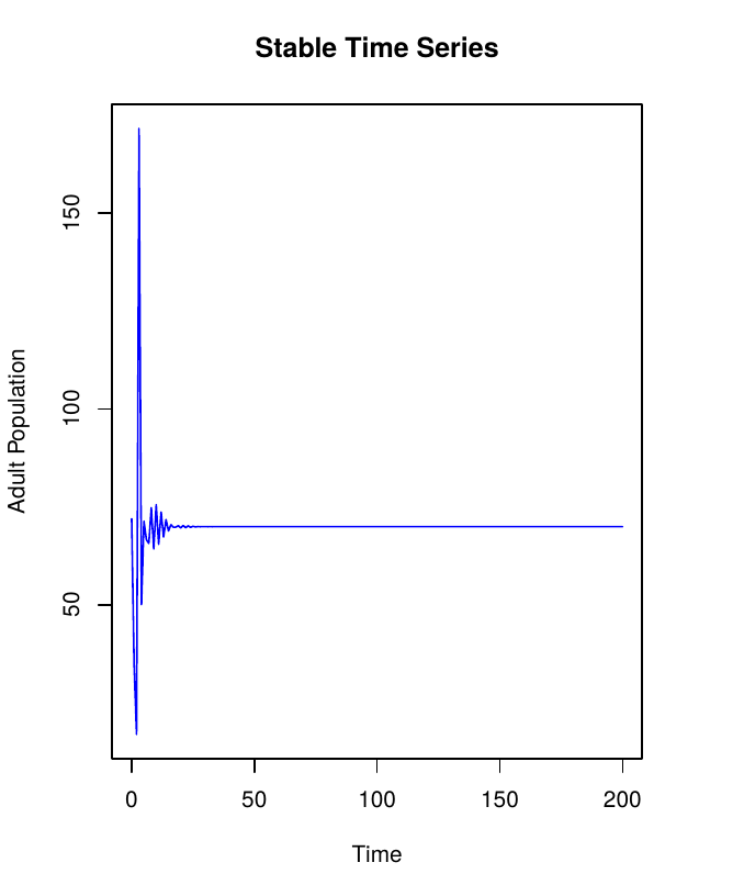
First, we programmed a function to create 200 aperiodic time series and 200 stable time series. The same fixed parameters as outlined in the paper were used along with μ_a = 0.73 for stable time series and μ_a = 0.96 for aperiodic time series. The starting value of larvae L_t, pupae P_t and adults A_t for each time series was randomized. The following equations were used to model the values of larvae, pupae and adult beetles respectively.

\begin{equation} \begin{array}{l} L_{t+1}=b \cdot A_{t} \cdot \exp \left(-c_{e a} A_{t}-c_{e \ell} L_{t}+E_{1 t}\right) \\ P_{t+1}=L_{t}\left(1-\mu_{\ell}\right) \exp \left(E_{2 t}\right) \\ A_{t+1}=\left(P_{t} \exp \left(-c_{p a} A_{t}\right)+A_{t}\left(1-\mu_{a}\right)\right) \exp \left(E_{3 t}\right) \end{array} \end{equation}

Each time series was then converted to a row vector and appended to the data frame Time_Series_Data which contains all 400 time series required to do analysis.

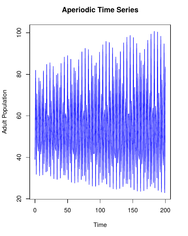
First, create 200 aperiodic time series.

Aperiodic Time Series

            
Time_Series_Data<- data.frame()
for (i in 1:200){
  parameters2 <- c(b = 7.48, c_ea = 0.009, c_pa = 0.004, c_el = 0.012, u_p = 0, u_l = 0.267, u_a = 0.96)

  state2 <- c(L = sample(2:100,1), P = sample(2:100,1), A = sample(2:100,1))

  beetles2<-function(t, state, parameters) {
    with(as.list(c(state, parameters)),{

      L1 <- b * A * exp((-c_el * L) - (c_ea * A))
      P1 <- L * (1 - u_l) 
      A1 <- (P * exp(-c_pa * A) + A * (1 - u_a)) 
      
      list(c(L1, P1, A1))
    })
  }


Aperiodic_i <- ode(y = state2, times = seq(0, 200), func = beetles2, parms = parameters2, method = "iteration")
  

aperiodic <- as.data.frame(Aperiodic_i) %>% select(A)

transposeAperiodic <- t(aperiodic) # Turns Column Vector into Row Vector

Time_Series_Data <- rbind.data.frame(transposeAperiodic,Time_Series_Data) 
}

Next, create 200 stable time series.

Stable Time Series

            
for (i in 1:200){
  parameters1 <- c(b = 7.48, c_ea = 0.009, c_pa = 0.004, c_el = 0.012, u_p = 0, u_l = 0.267, u_a = 0.73)

  state1 <- c(L = sample(2:100,1), P = sample(2:100,1), A = sample(2:100,1))
  
  beetles1<-function(t, state, parameters) {
    with(as.list(c(state, parameters)),{

      L1 <- b * A * exp((-c_el * L) - (c_ea * A))
      P1 <- L * (1 - u_l) 
      A1 <- (P * exp(-c_pa * A) + A * (1 - u_a)) 
      

      list(c(L1, P1, A1))
    }) 
  }

  
  Stable_i <- ode(y = state1, times = seq(0, 200), func = beetles1, parms = parameters1, method = "iteration")
  
stable <- as.data.frame(Stable_i) %>% select(A)
transposeStable<-t(stable)
Time_Series_Data <- rbind.data.frame(transposeStable,Time_Series_Data)
}

Now all 400 time series have been created, transposed into row vectors and added to the data frame Time_Series_Data which contains all 400 time series.

For ease of identification name each time series aperiodic or stable.

            
(setattr(Time_Series_Data, "row.names", c(rep("Stable",200),rep("Aperiodic",200))))

Part 2: Analysis of time series.

K-means clustering

The k-means clustering algorithm was used to show comparison between persistent homology and a more traditional classification method. Using the k-means clustering algorithm we attempt to correctly classify the time series data into two clusters: aperiodic and stable.

            
set.seed(250)
kmtotal <- kmeans(Time_Series_Data, 2, iter.max = 10, nstart = 1)

#Confusion matrix
km_clusters <- kmtotal$cluster
correct <- rep(c("1","2"), each=200)
cfm <- table(correct,km_clusters)

In order to analyse the results of the k-means clustering algorithm we create a confusion matrix which shows the number of true positives, true negatives, false positives, and false negatives.

\begin{aligned} &\begin{array}{rr} \text {} & + & - \\ Stable & 200 & 0 \\ Aperiodic & 119 & 81 \end{array} \end{aligned}

From the confusion matrix above it can be seen that all 200 stable time series are correctly clustered. However, only 81 of the aperiodic time series are correctly classified.

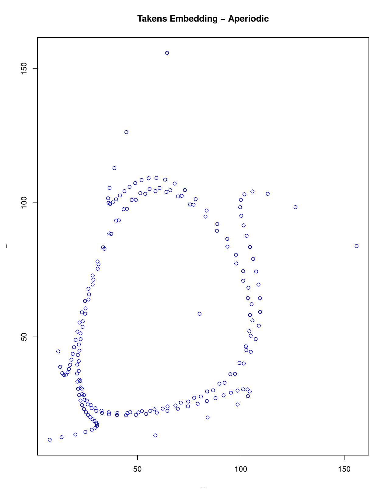
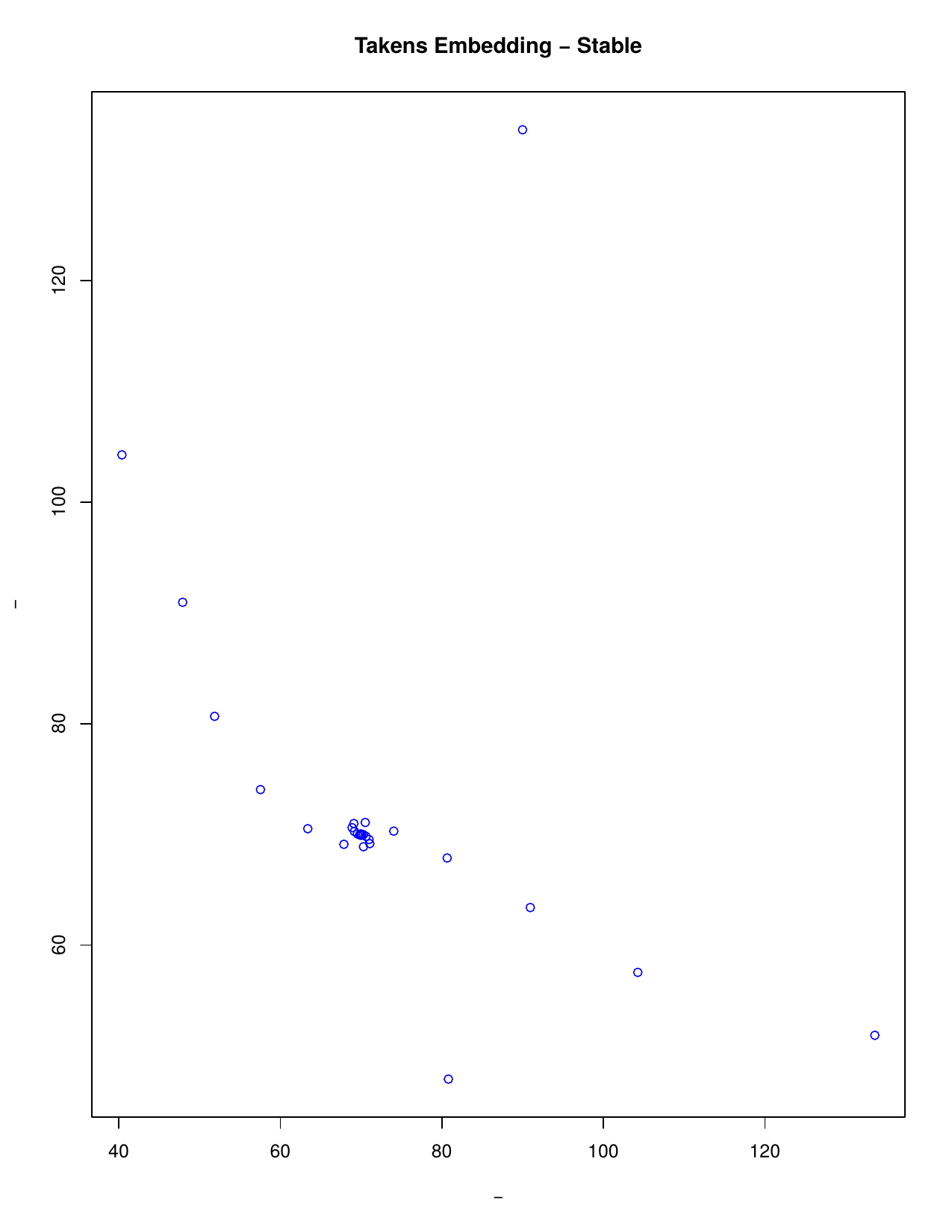
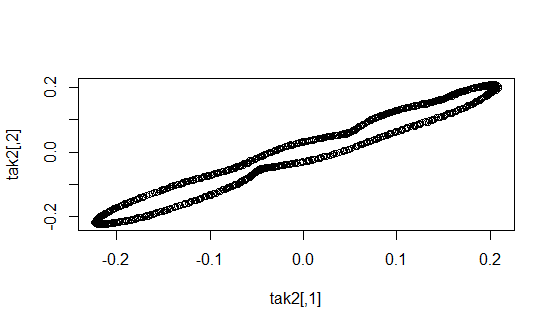
Takens' Theorem

Let \(M\) be a compact \(C^2\) differentiable manifold of dimension \(m\). Let \(\Phi: M \rightarrow M\) be a \(C^2\) diffeomorphism and let \(\mu: M \rightarrow \mathbb{R}\) be any \(C^2\) map. It is a generic property that the mapping \begin{equation} \Phi_{\phi, \mu}: M \rightarrow \mathbb{R}^{2 m+1}, x \mapsto\left(\mu(x), \mu \phi(x), \mu \phi^{2}(x), \ldots, \mu \phi^{2 m}(x)\right) \end{equation} is an embedding.

Takens’ embedding theorem states that we can reconstruct a time series considering time delays. A series can be reconstructed in phase space where m is the embedding dimension (the smallest dimension required to embed an object) and t the time delay. Thus, instead of analysing the series along time, we analyse its trajectory as a set of visited states in an m-dimensional Euclidean space. This is particularly useful to extract the topological behaviour we are interested in.

In the study of dynamical systems, a delay embedding theorem gives the conditions under which a chaotic dynamical system can be reconstructed from a sequence of observations of the state of a dynamical system. The reconstruction preserves the properties of the dynamical system that do not change under smooth coordinate changes (i.e., diffeomorphisms), but it does not preserve the geometric shape of structures in phase space.

The theorem motivates the idea of studying a time series x₁, x₂, x₃, ... by choosing some embedding dimension m and forming the sequence of m-dimensional vectors v₁=(x₁, x₂, ...,x_m), v₂=(x₂, x₃, ..., x_m+1), v₃=(x₃, x₄, ..., x_m+2), ... Then the geometry of the m-dimensional vectors v₁, v₂, v₃, ... can be studied using a range of techniques. One technique involves creating filtered simplicial complexes and applying persistent homology to them. A filtered simplicial complex is just a sequence of inclusions K₁ >--> K₂ >--> K₃ >--> ... of simplicial complexes K_i.

Takens Embedding of Aperiodic Time Series

Simplicial Complexes

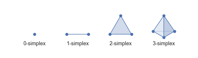
A simplex is a generalization of the notion of a triangle or tetrahedron to arbitrary dimensions.

a 0-simplex is a point,
a 1-simplex is a line segment,
a 2-simplex is a triangle,
a 3-simplex is a tetrahedron,

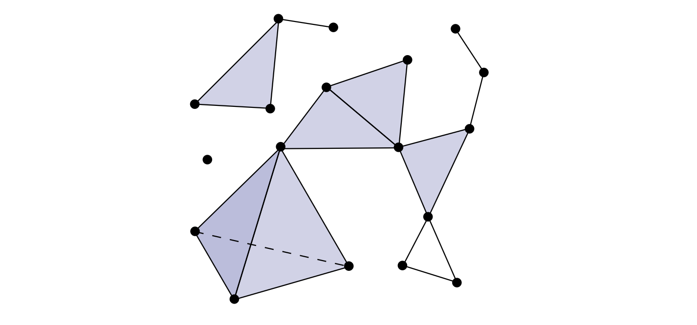
In topology and combinatorics, it is common to “glue together” simplices to form a simplicial complex.

A simplicial complex, as seen below, is a union of simplices satisfying certain conditions.

Betti Numbers

In algebraic topology, Betti numbers are used to distinguish topological spaces based on the connectivity of n-dimensional simplicial complexes.

Betti number: B_n = dim(ker(d_n))-dim(image(d_n+1))

Informally, the kth Betti number refers to the number of k-dimensional holes on a topological surface. The first few Betti numbers have the following definitions for 0-dimensional, 1-dimensional, and 2-dimensional simplicial complexes:

b₀ is the number of connected components
b₁ is the number of one-dimensional or "circular" holes
b₂ is the number of two-dimensional "voids" or "cavities"

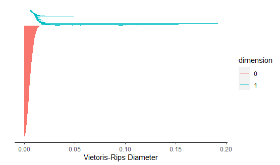
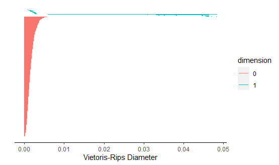
Persistent Homology: Bar Codes and Persistence Diagrams

To any simplicial complex K we can associate a homology vector space H_n(K). To a filtered simplicial complex K₁ >--> K₂ >--> K₃ >--> ... we can associate a sequence of linear homomorphisms H_n(K₁) --> H_n(K₂) --> H_n(K₃ ) --> .... This sequence of linear homomorphisms can be fully captured using the language of persistent n-dimensional Betti numbers.

Persistent homology is a method for computing topological features of a space at different spatial resolutions. The space must first be represented as a simplicial complex. More persistent features are detected over a wide range of spatial scales and are deemed more likely to represent true features of the underlying space rather than noise.

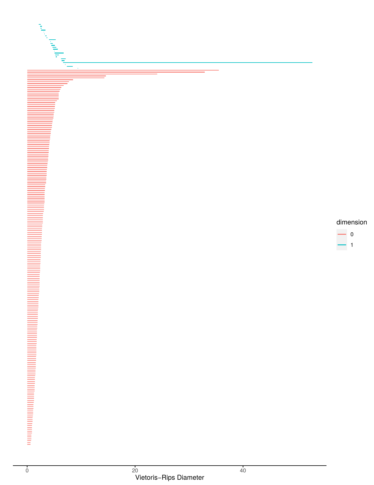
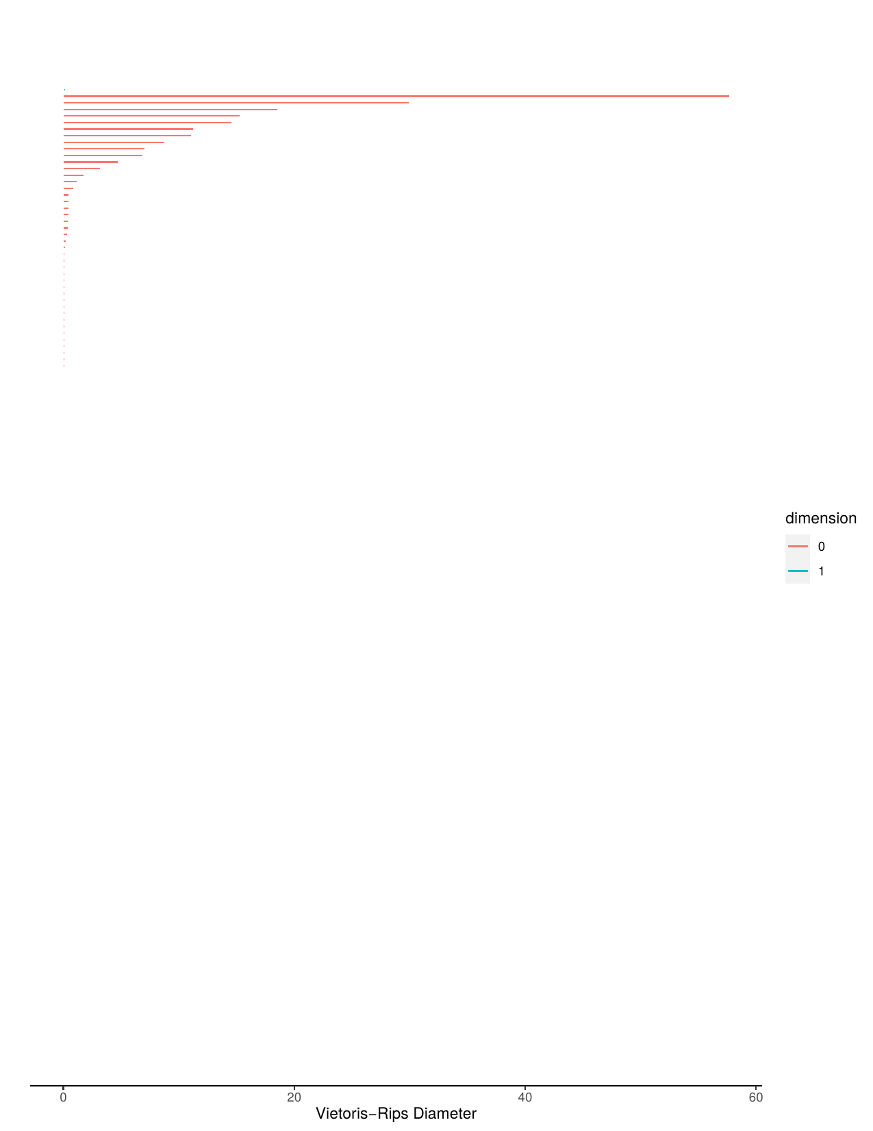
A bar code is a visual representation of persistent homology. Long bars represent features and short bars represent noise.

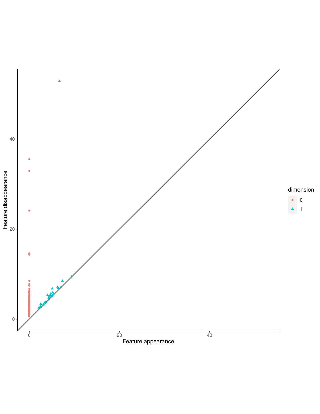
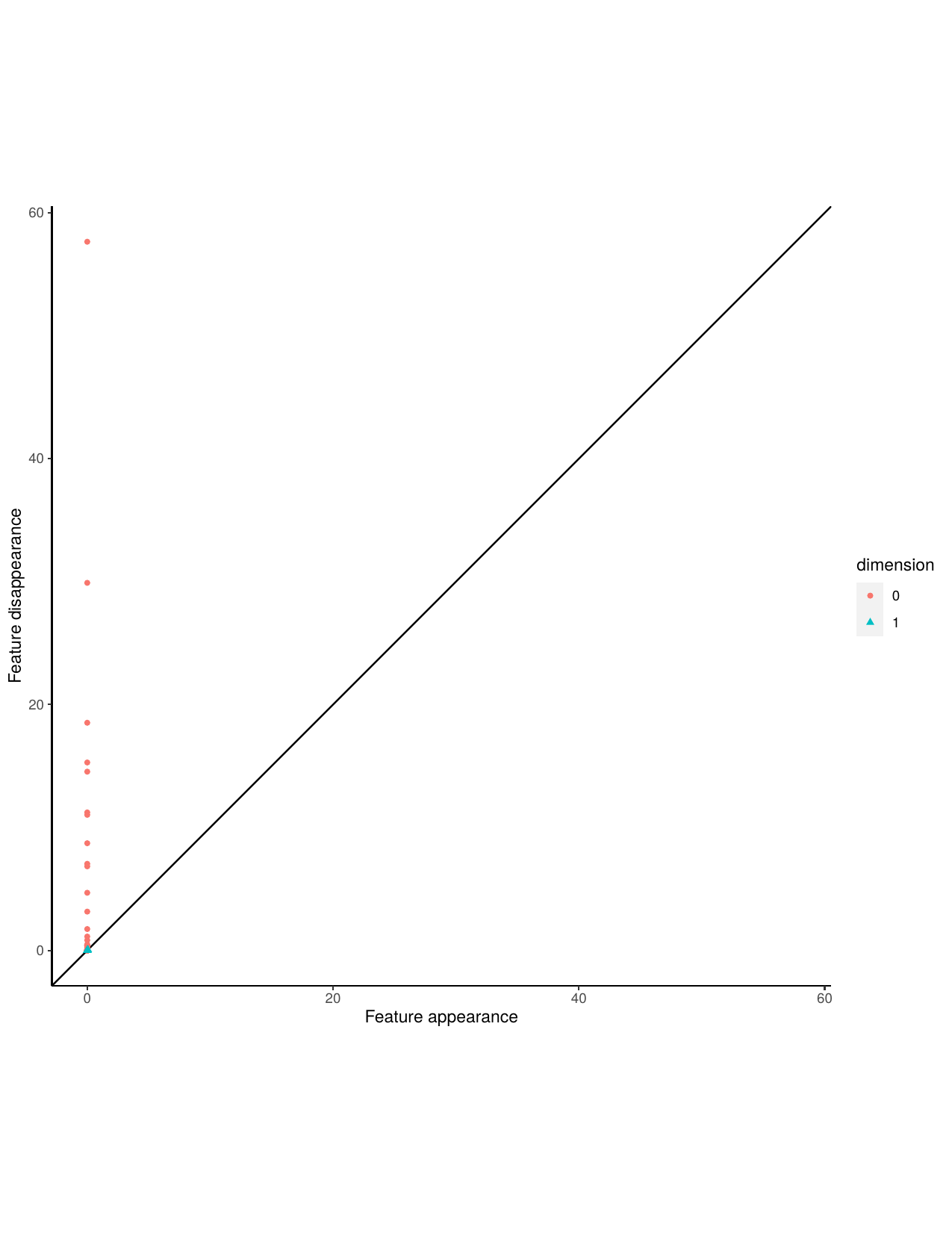
A persistence diagram is very similar to a barcode, it captures the birth and death of features. The x-coordinate of a point represents when that point was born and the y-coordinate represents when that feature died. Features that are short lived occur close to the 45 degree line, while more persistent features occur at a greater distance from the 45 degree line.

If you would like more information about persistent homology please view this paper.

Aperiodic barcode and stable barcode.

Aperiodic persistence diagram and stable persistence diagram.

Next, we construct a Takens embedding and calculate persistent homology and Betti numbers for the stable time series. Then sort the data by correct and incorrect classifications.

        
pers_stable <- data.frame()
for (i in 1:200){
    x<- data.matrix(Time_Series_Data[i,])
    a<- buildTakens(x,2,3)

    hom <- calculate_homology(a,return_df = TRUE)
    hom <- hom %>%
        mutate(persistence = death-birth) %>%
        mutate(persistent = ifelse(persistence > max(persistence)-0.00001, 1,0))

    hom_matrix <- data_frame(hom) %>% select(dimension, persistent)
    hom_matrix <- as.data.frame(hom_matrix) 
    p1 <- hom_matrix[hom_matrix$persistent == '1',] 
    pers_stable <- rbind.data.frame(pers_stable,p1) 


#Sort the data by correct and incorrect classifications        
check_stable <- pers_stable[pers_stable$dimension == 0,]
stable_correct_hom <- nrow(check_stable)
stable_incorrect_hom <- 200 - stable_correct_hom

Do the same for the aperiodic time series.

        
pers_aperiodic <- data.frame()
for (i in 201:400){
    x1<- data.matrix(Time_Series_Data[i,])
    a1<- buildTakens(x1,2,3)
    hom1 <- calculate_homology(a1,return_df = TRUE)
    hom1 <- hom1 %>%
    mutate(persistence = death-birth) %>%
    mutate(persistent = ifelse(persistence > max(persistence)-0.00001, 1,0))
    hom_matrix1 <- data_frame(hom1) %>% select(dimension, persistent)
    hom_matrix1 <- as.data.frame(hom_matrix1) 
    p2 <- hom_matrix1[hom_matrix1$persistent == '1',] 
  
    pers_aperiodic <- rbind.data.frame(pers_aperiodic,p2)  
}

    #Sort the data by correct and incorrect classifications
    check_aperiodic <- pers_aperiodic[pers_aperiodic$dimension == 1,] 
    aperiodic_correct_hom <- nrow(check_aperiodic)
    aperiodic_incorrect_hom <- 200 - aperiodic_correct_hom

We can analyse the results of persistent homology using a confusion matrix. This allows for easy comparison with k-means clustering.

        
cfm_hom <-cbind(c(stable_correct_hom,aperiodic_incorrect_hom),c(stable_incorrect_hom,aperiodic_correct_hom))

\begin{aligned} &\begin{array}{rr} \text {} & + & - \\ Stable & 200 & 0 \\ Aperiodic & 19 & 181 \end{array} \end{aligned}

From the confusion matrix above it can be seen that all 200 stable time series and 181 of aperiodic time series are correctly clustered.

Part 3: Conclusion from first example

Persistent homology is more effective at classifying the given time series data than k-means clustering. Both k-means clustering and persistent homology classify all 200 stable time series correctly. However, there is quite a significant difference when it comes to classifying aperiodic time series. K-means clustering only correctly classifies 81 aperiodic time series whereas persistent homology correctly classifies 181 aperiodic time series. This shows how effective persistent homology is over k-means clustering at classifying the given time series data

This example shows how effective topology can be and how it can be considered for use as an extra tool for statistics.

Our full R code can be found here.

Second Example: Musical Instrument Classification

Another application of persistent homology can be seen in The University of Colorado paper “Computational Topology Techniques for Characterizing Time-Series Data” which analyses time series data and shows as an example how persistent homology can be used to classify notes from different musical instruments.

Our aim is to use this idea to try to correctly classify an instrument by its note. For our analysis we use two instruments: flute and clarinet. By taking samples of note A4 from each instrument we use persistent homology to try to correctly predict whether it is flute or clarinet.

Part 1: Constructing the Time Series

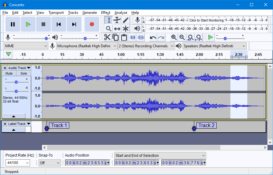
To carry out our analysis we had to generate time series data for flute and clarinet. We used the University of New South Wales Music Science audio file bank for our instrument samples. For both flute and clarinet, we used note A4. We imported the audio files into Audacity in order to analyse each instrument. The files were then processed through audacity and the sample data export function generated a time series for each note. The time series for both flute and clarinet were then exported to a CSV file and imported into R.

Below shows a sample audio file output from Audacity. The time series, as clearly seen in the track bar below, can be exported to a CSV file and imported into R.

Part 2: Analysis of time series

The following R Libraries were required.

            
library(nonlinearTseries)
library(TDAstats)
library(tidyverse)
library(data.table)

For each instrument we start by taking 30 sample time series that have random starting points and each being 1000 points long or roughly .05 seconds of the full time series. We start by computing the average B₁ number for the flute. Using the 30 samples, we construct a Takens embedding and calculate homology for each sample. We then record the number of one-dimensional holes for each sample and compute the average B₁ number for the flute. This will be used in the classification of our data.


#get average betti number for flute
average_list_flute <- c()
Flute_full_note <- read.csv("FluteAfull.csv")
for (i in 1:30) {
  ai <- sample(1:37999,1,replace = FALSE, prob = NULL)
  bi <- ai + 1000
  sample_sequence_ai <- Flute_full_note[ai:bi,]
  
  Flute_homology <- data.frame()
  
  flute_A4_matrix <- data.matrix(sample_sequence_ai)
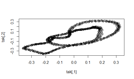
  tak <- buildTakens(flute_A4_matrix,2,3)
  hom <- calculate_homology(tak,return_df = TRUE) 
  hom_matrix <- calculate_homology(tak,return_df = FALSE) 
  hom <- hom %>%
    mutate(persistence = death-birth) %>%
    mutate(persistent = ifelse(persistence > 0.029, 1,0))
  hom_matrix <- data.frame(hom) %>% select(dimension, persistent)
  hom_matrix <- as.data.frame(hom_matrix) 
  p1 <- hom_matrix[hom_matrix$persistent == '1',] 
  Flute_homology<-rbind.data.frame(Flute_homology,p1)
  avg <- nrow(Flute_homology)
  average_list_flute <- append(average_list_flute,avg)
}


avg_betti_number_flute <- sum(average_list_flute)/length(average_list_flute)

The average B₁ number for flute is 3.

Next, we repeat the same steps to calculate the average B₁ number for the clarinet.


#clarinet
average_list_clarinet <- c()
Clarinet_full_note <- read.csv("ClarinetAfull.csv")
for (i in 1:30) {
  ai2 <- sample(1:95000,1,replace = FALSE, prob = NULL)
  bi2 <- ai2 + 1000
  sample_sequence_ai2 <- Clarinet_full_note[ai2:bi2,]
  
  Clarinet_homology <- data.frame()
  
  Clarinet_A4_matrix <- data.matrix(sample_sequence_ai2)
  tak2 <- buildTakens(Clarinet_A4_matrix,2,3)
  hom2 <- calculate_homology(tak2,return_df = TRUE) 
  hom_matrix2 <- calculate_homology(tak2,return_df = FALSE) 
  hom2 <- hom2 %>%
    mutate(persistence = death-birth) %>%
    mutate(persistent = ifelse(persistence > 0.029, 1,0))
  hom_matrix2 <- data.frame(hom2) %>% select(dimension, persistent)
  hom_matrix2 <- as.data.frame(hom_matrix2) 
  p2 <- hom_matrix2[hom_matrix2$persistent == '1',] 
  Clarinet_homology<-rbind.data.frame(Clarinet_homology,p2)
  avg2 <- nrow(Clarinet_homology)
  average_list_clarinet <- append(average_list_clarinet,avg2)
}


avg_betti_number_clarinet <- sum(average_list_clarinet)/length(average_list_clarinet)

The average B₁ number for clarinet is 1.

Now we have the average B₁ number for both flute and clarinet.

Next, we want to create a test data set consisting of 30 flute time series samples and 30 clarinet time series samples.

            
#make flute testing data
Flute_full_note <- read.csv("FluteAfull.csv")
Flute_test_data <- data.frame()
for (i in 1:30) {
  xi11 <- sample(1:37999,1,replace = FALSE, prob = NULL)
  yi11 <- xi11 + 1000
  sample_sequence_xi11 <- Flute_full_note[xi11:yi11,]
  
  Flute_dataframe <- as.data.frame(sample_sequence_xi11)
  Flute_A_transpose <- t(Flute_dataframe)
  Flute_test_data <- rbind.data.frame(Flute_A_transpose,Flute_test_data)
}

#make clarinet testing data
Clarinet_full_note <- read.csv("ClarinetAfull.csv")
Clarinet_test_data <- data.frame()
for (i in 1:30) {
  xi12 <- sample(1:94999,1,replace = FALSE, prob = NULL)
  yi12 <- xi12 + 1000
  sample_sequence_xi12 <- Clarinet_full_note[xi12:yi12,]
  
  CLarinet_dataframe <- as.data.frame(sample_sequence_xi12)
  Clarinet_A_transpose <- t(CLarinet_dataframe)
  Clarinet_test_data <- rbind.data.frame(Clarinet_A_transpose,Clarinet_test_data)
}

Join flute test data and clarinet test data into one data frame and label each row.

            
test_data_set<- rbind(Flute_test_data,Clarinet_test_data)
(setattr(test_data_set, "row.names", c(rep("Flute",30),rep("Clarinet",30))))

Using the test data set we attempt to classify each time series into either flute or clarinet. Starting with the first 30 rows corresponding to flute, if the B₁ number for each time series is close the average B₁ number for flute we computed earlier it is classified as flute.

            
#analyse flute
flute_assign <- c()
clarinet_assign <- c()
for (i in 1:30) {
  test_flute_data_row <- test_data_set[i,]
  
  Flute_homology1 <- data.frame()
  
  test_flute_matrix <- data.matrix(test_flute_data_row)
  tak11 <- buildTakens(test_flute_matrix,2,3)
  hom11 <- calculate_homology(tak11,return_df = TRUE) 
  hom_matrix11 <- calculate_homology(tak11,return_df = FALSE) 
  hom11 <- hom11 %>%
    mutate(persistence = death-birth) %>%
    mutate(persistent = ifelse(persistence > 0.029, 1,0))
  hom_matrix11 <- data.frame(hom11) %>% select(dimension, persistent)
  hom_matrix11 <- as.data.frame(hom_matrix11) 
  p11 <- hom_matrix11[hom_matrix11$persistent == '1',] 
  Flute_homology1 <-rbind.data.frame(Flute_homology1,p11)
  
  avg <- nrow(Flute_homology1)
  if (avg < 1.2){
  clarinet_assign <- append(clarinet_assign,1)
  } else {
    flute_assign <- append(flute_assign,1)
}
}

Compute the number of correct and incorrect flute classifications.

            
correct_flute <-length(flute_assign)
incorrect_flute <- 30-length(flute_assign)

Again, using the test data set we attempt to classify each time series into either flute or clarinet. This time using the last 30 rows which corresponds to clarinet, if the B₁ number for each time series is close the average B₁ number for clarinet we computed earlier it is classified as clarinet.

            
#analyse clarinet
flute_assign1 <- c()
clarinet_assign1 <- c()
for (i in 31:60) {
  test_clarinet_data_row <- test_data_set[i,]
  
  Clarinet_homology1 <- data.frame()
  
  test_clarinet_matrix <- data.matrix(test_clarinet_data_row)
  tak12 <- buildTakens(test_clarinet_matrix,2,3)
  hom12 <- calculate_homology(tak12,return_df = TRUE) 
  hom_matrix12 <- calculate_homology(tak12,return_df = FALSE) 
  hom12 <- hom12 %>%
    mutate(persistence = death-birth) %>%
    mutate(persistent = ifelse(persistence > 0.029, 1,0))
  hom_matrix12 <- data.frame(hom12) %>% select(dimension, persistent)
  hom_matrix12 <- as.data.frame(hom_matrix12) 
  p12 <- hom_matrix12[hom_matrix12$persistent == '1',] 
  Clarinet_homology1 <-rbind.data.frame(Clarinet_homology1,p12)
  
  avg1 <- nrow(Clarinet_homology1)
  if (avg1 < 1.2){
    clarinet_assign1 <- append(clarinet_assign1,1)
  } else {
    flute_assign1 <- append(flute_assign1,1)
  }
}

Compute the number of correct and incorrect clarinet classifications.

            
correct_clarinet <- length(clarinet_assign1)
incorrect_clarinet <- 30 - length(clarinet_assign1)

Create a confusion matrix to analyse the results.

            
cfm <-cbind(c(correct_flute,incorrect_clarinet),c(incorrect_flute,correct_clarinet))

\begin{aligned} &\begin{array}{rr} \text {} & + & - \\ Flute & 24 & 6 \\ Clarinet & 0 & 30 \end{array} \end{aligned}

The confusion matrix above shows 24 flute samples correctly classified and all 30 clarinet samples correctly classified.

Part 3: Conclusion from second example.

Persistent homology is quite effective at classifying the given time series data.

By constructing a Takens embedding, persistent homology can distinguish between flute and clarinet and it classifies all 30 clarinet time series correctly and 24 flute time series correctly.

In the paper the authors also tried using a classical classification involving fast Fourier transforms. The classical approach was not as successful as the persistent homology approach.

This example again shows how effective topology can be and how it can be considered for use as an extra tool for statistics.

Our full R code can be found here.

Overall conclusion

The investigations conducted on data from flour beetle populations and musical instruments based on two recent research papers "Persistent homology for time series and spatial data clustering" - Cássio M.M. Pereira/Rodrigo F. de Mello and “Computational Topology Techniques for Characterizing Time-Series Data” - University of Colorado show how persistent homology can be used for time series classification.

The usefulness and effectiveness of persistent homology at classifying time series can be clearly seen even in comparison to more traditional methods such as k-means clustering. Overall topology can be very effective and it can be considered for use as an extra tool for statistics.

Topological Data Analysis - The use of persistent homology for time series classification.

Introduction

Aim

Background

What is a Time Series?

First Example: Population growth analysis of Tribolium flour beetle.

Part 1: Construct time series.

Aperiodic Time Series

Stable Time Series

Part 2: Analysis of time series.

K-means clustering

Takens' Theorem

Simplicial Complexes

Betti Numbers

Persistent Homology: Bar Codes and Persistence Diagrams

Part 3: Conclusion from first example

Second Example: Musical Instrument Classification

Part 1: Constructing the Time Series

Part 2: Analysis of time series

Part 3: Conclusion from second example.

Overall conclusion